Here we will go through how Excel is structured, where you will find important and smart functions, and various peculiarities you should know. In short, we’ll show you how to make the program work for you, so to speak, to ensure a smooth user experience.
An introduction to Excel’s interface
To work effectively in any program, you need to have an idea of what functions are available and where to find them. Excel is a sophisticated program with hundreds or even thousands of functions. But of course they are not all in a row; by learning the structure, you can find more functions when you need them.
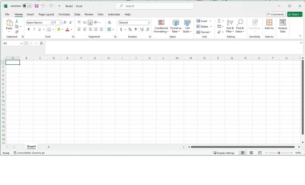
Like Word, Excel uses a layout where many, if not most, functions are located in the so-called Ribbon: the toolbar at the top of the program window, divided into tabs such as Home, Insert, and Data.
Foundry
Unlike Word, you don’t necessarily have to rummage around in these tabs, and many users have barely looked in tabs other than Start and Insert. However, there’s a lot to pick up if you start exploring them.
- Home: Basic formatting and shortcuts to commonly used functions like AutoSum and Filter.
- Insert: When you want a chart, table, image, or text box.
- Page Layout: Only if you are going to print.
- Formulas: One of Excel’s most important features is all the built-in mathematical formulas, and this tab helps you find formulas based on areas such as finance, text, and math.
- Data: Mainly for connecting to external data sources such as databases, but also has some features useful to anyone.
- Review: Is someone other than you going to work in a document, or will you continue to use the same document for a long time? Then comments and tracking are very useful, and you can find them here.
- View: In addition to previewing for printing, you can lock the first row and/or column, which can be very useful in a large table. There are also settings here to display the open spreadsheet in multiple windows so you can look in several places at once.
What we think you’ll notice as you become more familiar with Excel, however, is that you’ll rarely need to leave the Home tab. Almost all the functions in the other tabs either have keyboard shortcuts or are formulas you can learn.
Rearrange the menus
Do you find the order of commands in the menus impractical, or are you missing some handy feature? Excel has great options for setting what to include and in what order.
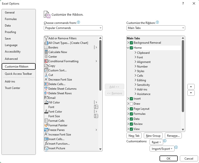
Right-click in a blank space anywhere in the Ribbon and select Customize Ribbon, or select File > Options and click on Customize the ribbon.
Foundry
On the right side of the dialogue box, you will find the existing content and layout of the Ribbon. There you can add new tabs and groups inside tabs, but also reorder what is already there. For example, say you are not using Styles-functions in the Home tab very often, but you do use the Editing functions like AutoSum and Sort and Filter. Then you can simply grab and drag Styles so it is last in the list under Home. Press OK and Excel will save the change.
In the list on the left you will normally find Popular Commands but if you’re looking to add handy features that are not there you can select Commands not in the Ribbon in the drop-down menu under Choose commands from.
Spreadsheet
The bulk of the work in Excel is done in the grid of cells in rows and columns that make up the spreadsheet itself. This is where you build tables, fill in formulas, and rearrange, sort, and make sense of data. Make friends with this grid — it makes everything easier.
The grid starts at the top left with row 1, column A. You don’t have to start there, you can put numbers and other things in any cells you like. New documents are created with a blank sheet called Sheet1 — you add new ones by pressing the plus button at the bottom left of the program window. Each sheet can handle a maximum of 1,048,576 rows and 16,384 columns. Each cell can contain a maximum of 32,767 characters and 253 line breaks. You always have plenty of room, to say the least.
Wherever you are in the grid, you can see row and column numbers, and these have several important functions.
Foundry
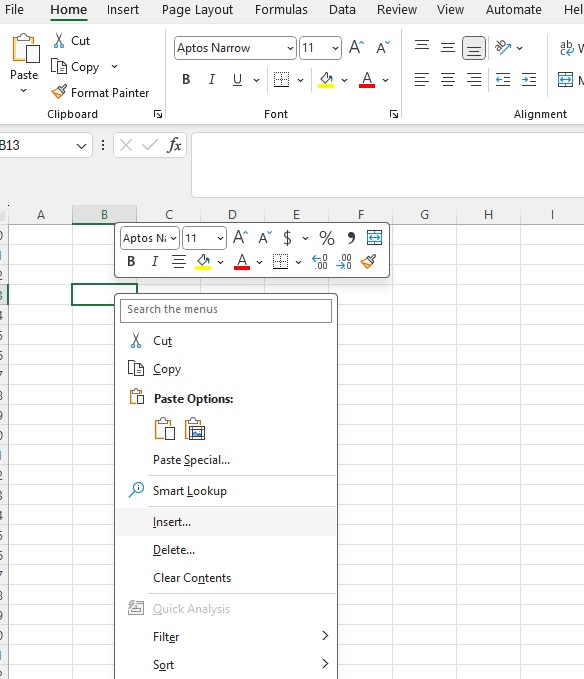
Right-click on one of these row or column numbers. For example, in the context menu that appears, you will find the functions Insert and Delete. Insert adds a new row or column above or to the left of what you clicked on, and moves all content one step down or to the right. Formulas that reference a particular cell are automatically changed when you do this — you don’t need to go in and change anything yourself.
If you have copied or cut one or more cells before right-clicking, Insert is replaced by Paste copied/cut cells. Depending on how you copied, this may move only some rows/columns or all of them.
Click on one of the numbers and the whole of that row or column will be selected. You can use this to copy all the content in it, for example, or to change the format of the content. A typical use is when you want to paste numbers, text, and dates into a column and don’t want Excel to format these differently but just as plain text.
How number formats work in Excel
A cell in Excel can contain different kinds of data, which in turn can be formatted in different ways. You can see what format a cell has by selecting it and looking in the Numbers section in the Home tab. It is important to understand the difference between what the content looks like and what it actually is.
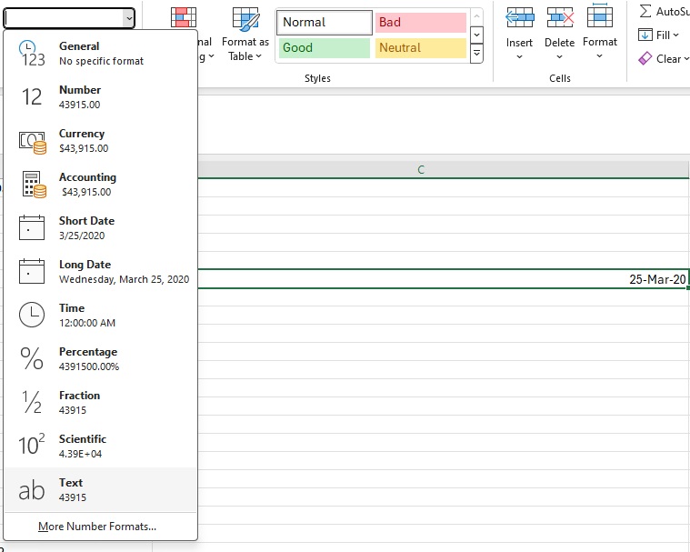
Take dates, for example. When you enter a date in a blank cell that has the number format General, Excel recognizes it and automatically changes the number format to Date. Select the cell and click on the drop-down menu where it now says Date. You can see here that if you switch to the Text format, the content will be displayed as a number. 25 March 2020, for example, becomes 43915.
Foundry
This is because dates are internally stored as numbers where “1” means 1 January 1900. You cannot use dates earlier than that in Excel, so genealogists and others will have to work around it by, for example, using text format instead of date format. You can still sort in date order as long as you follow the ISO standard of year-month-day, but you cannot use such cells in calculations of, for example, the number of days between two dates. Such problems can also be overcome, but it is too advanced for this guide.
Formulas
You can of course use Excel only to manually enter text, dates, and numbers in tables. But the usefulness of the program comes from writing formulas that retrieve data from other cells, perform calculations of various kinds, and put the results in their cell.
As long as you don’t create circle references (where the contents of one cell depend on the contents of a cell whose contents depend on the contents of the first cell), you can have formulas that reference formulas that reference formulas — and so on. Make a change at the beginning of the chain and the results change all the way to the last step.
A formula always starts with an equal sign. After that, you do not write mathematical formulas according to Excel’s special syntax. It’s similar to regular math, but it’s still its own thing.
=PMT(B6/12;B8*12;B4)
=OM(H8>250000; (H8-250000)*0,05; 0)+OM(H8>175000;OM(H8>
References to cells are written with the letter of the column followed by the row number, for example B6 or H8. An important thing to learn is the difference between a relative reference and an absolute one.
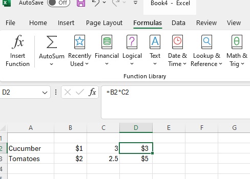
Say you are building a table with prices, quantities, and costs: For example, Cucumber – $1/piece – 3 pieces – $3. You might fill in the first three columns manually, but the last one is suitable for a formula. If it says Cucumber in A2, $1 in B2, and 3 in C2, you can fill in the following formula in D2: =B2*C2.
Foundry
If you then fill in A3: Tomatoes, B3: $2/pound, C3: 2.5 pounds, you can copy D2 and paste it into D3 and Excel will automatically fill in the correct formula: =B3*C3. This is called a relative reference.
By placing dollar signs on both sides of the column letter (for example $B$2), the reference becomes absolute. This means that if you copy the formula and paste it into another cell, that reference will still be to the exact same cell. For example, this could be a cell where you enter an interest rate to be used in many places in a table. You can mix relative and absolute references in a formula.
We can go a bit deeper into how to use advanced math in Excel, for example to calculate with roots and exponents, which are common in economics. A simple example: Calculate what the daily interest rate is if the annual interest rate is 2.5 percent using the formula =(1+A1)^(1/365)-1 (in A1 you have filled in 2.5% or 0.025).
How to use data from Excel in Word documents
Excel has its own functions for simple layout, but if you are writing a report or similar and want to use data from large Excel tables, it’s easy to link the two Office programs.
Foundry
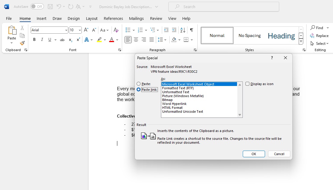
If you have very simple data or simply prefer to format tables in Excel, you can select what you want and simply paste it into Word. However, this means that you will have to make any changes manually in Word. If you want to be able to have up-to-date figures and charts, it’s much more practical to link or embed.
- Start by selecting what you want to paste into Excel.
- Open the Word document and place the pointer in the right place.
- Select the Paste > Paste special.
- Select the As: Microsoft Excel spreadsheet object.
- Select either Paste or Paste link on the left.
The former means that a copy of the content is inserted directly into Word and you can edit it there. The latter means that you create a link to that part of the Excel sheet and to make changes you have to do it in Excel.
Linked content can be very useful if you have a large, complicated spreadsheet in Excel and want to paste just the result of all the calculations, either a table or a chart. Then you can go in and add, delete or change data in Excel and get updated results in Word.
Learn keyboard shortcuts
Excel is full of keyboard shortcuts and if you watch a veteran user work, you’ll probably find that they very rarely reach for the mouse. You can do almost anything you can think of with the keyboard alone, and it’s often quicker than rummaging through menus with the mouse.
We don’t have space to go through all the handy keyboard shortcuts, but here’s a small selection of the most useful commands that are unique to Excel (copy, paste, select all, and the like you probably already know):

- Tab – when you start filling in a formula, Excel displays a list of suggestions. Use the arrow key to select the right one and press Tab to fill it in. For example, you can type a long formula name like NET WORKING DAYS faster.
- F4 – toggles between relative and absolute references for the cell reference you have the pointer in, so you don’t have to type dollar signs. The order is relative -> absolute row and column -> absolute row -> absolute column.
- F2 – edit the selected cell.
- Alt-Return – insert row break in a cell.
- Ctrl-D – first select a number of cells in one or more columns. Ctrl-D then copies the contents of the topmost cell of each selected column to the selected cells below it.
- Ctrl-Home followed by Shift-Ctrl-End – select the entire used area of the open sheet.
- Ctrl-arrow key – jump to the last cell with content before an empty cell, in the direction the arrow points.
- Shift-Ctrl-arrow key – select all cells with content starting from the cell you have now selected, in the direction of the arrow.
- Ctrl-H – open Find and Replace where you can quickly replace, for example, incorrect periods with commas and the like. Select a number of cells, rows, or columns beforehand to limit the function to these.
There are hundreds more. When you hover over a function in the menus, you can see that function’s keyboard shortcut, and you can also check out Microsoft’s list here.
This article was translated from German to English and originally appeared on pcforalla.se.
This article originally appeared on our sister publication PC för Alla and was translated and localized from Swedish.


